Review2: (08/24 - 09/25)

Algorithms:

Week 2:

• What’s the differences between KNN and KMeans?
  • Could you explain KNN/KMeans within 2 sentences?
  • How K affects the output from KNN/KMeans?
  • How do you choose K for KNN/KMeans?
• Random forests using a sub-sampling method to handle data too big to fit into RAM
  • Describe that method
  • Sub-sampling can miss some data. How does Random Forests reduce the odds of such misses?
  • How to make conclusions across the whole forest?
  • How to apply this heuristic to other learners?
• Naive Bayes classifiers divide their input rows according to the class variable, then collect different stats on each column for each class.
  • Let all boys smell like sugar and be 1 meter tall and have long hair
  • Let all girls smell like spice and be 2 meters tall and have short hair
  • Let all elephants smell like grass and be 3 meters tall and have very short hair
  • Given the above, describe the likelihood calculation for classifying a new thing that is 1.8 meters tall with short hair.
• Comment on the merits of KNN or NB or RF for incremental anomaly detection.
• Comment on the merits of KNN or NB or RF for incremental model building
• Explain in your words what is dominance? Please give one compare function to be used for dominant.
• Are all the learners explainable for their output/predictions? Give 2 example learners that are explainable, and 2 that aren’t.
• What are the common Evaluation Criteria for the learners? Why these criteria are important in the real world software engineering?

Notes: Pareto Domination

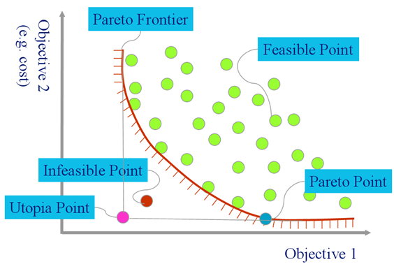
The human condition is a constant balancing act between vaguely understood, often competing, goals. For example:

In such trade-off diagrams, point on the Pareto frontier

Boolean domination says that I dominates J iff

• I is better on at least one objective, and worse on none.
• Cannot distinguishing between very near and very far dominance.
• Often gets confused by more than 3 objectives.

Indicator dominance sums the difference in the objective scores and shouts that out load (raises it to an exponential)

• Better for large number of objectives.

local function dominate1(i,j,t)
  local e,n = 2.71828,#t.goals
  local sum1,sum2=0,0
  for _,col in pairs(t.goals)  do
    local w= col.weight
    local x= NUM.norm(col, i.cells[col.pos])
    local y= NUM.norm(col, j.cells[col.pos])
    sum1 = sum1 - e^(w * (x-y)/n)
    sum2 = sum2 - e^(w * (y-x)/n) 
  end 
  return sum1/n < sum2/n end

Notes: K-means

Pick K centroids at random; label all data with their nearest centroid; for all things with same centroid, compute means; move centroids to that mean position; repeat

Notes: Mini-batch k-means

1. Data arrives in random order. Take the first “K” items, call them centroids (say, K-32);
2. Read next M items (say M=512)
   • Label each item with nearest centroid.
   • Add +1 to a centroid whenever some new item decides it is its nearest
3. Nudge each centroid by a weighted towards each item in the batch.
   • E.g. If centroid “weighs 250” then move it 1/250 th towards the item
4. Goto 2.

Decision Trees

See homework

Fast Frugal Decision Trees

referece

Extremely extremely simple decision trees.

• Binary classes
• Restricted to just a few levels (e.g. L=4)

2 nodes at each level.

• Leaf node: One for the attribute range A=R that most strongly predicts for something
• Base of sub-tree: other node holds all rows that do not have A=R

More than 2 classes? No problem. For each class, repeat for C and not C.

So fast we can run it N times with different internal thresholds to get a ROC curve.

PRISM:

Make a rule, throw away all the rows covered by the condition of that rule. Repeat on the remaining data.

• The result is a decision list (aka nested if then else) where rule[i] only applies if rules 1..i-1 are all false.

To make a rule of the form LHS ⇒ C (short form)

• Set LHS to empty.
• Find the attribute value Ai=Vi that predicts for any class C with highest accuracy. Add to LHS.
• For all data with Ai=Vi, add to the LHS add the range Aj=Vj which most improves accuracy. - If none found then then print LHS ⇒ C - and delete all rows with LHS
• Now go make another rule.

Full form:

For each class C
  Initialize E to the instance set
  While E contains instances in class C
    Create a rule R with an empty left-hand side that predicts class C
    Until R is perfect (or there are no more attributes to use) do
       For each attribute A not mentioned in R, and each value v,
          Consider adding the condition A = v to the left-hand side of R
          Select A and v to maximize the accuracy p/t
           (break ties by choosing the condition with the largest p)
       Add A = v to R
   Remove the instances covered by R from E
   Print R

t = total instances
p = positive instances

If applied to the weather data

Comapre with decision tree:

IMPORTANT NOTE: known to perform less-than-great unless you restrict Aj=Rj to “power ranges”; e.g. those with the above-median score from supervised discretization.

For a startof the art incremental rule learning (in the PRISM mode), see Very fast decision rules for classification in data streams, Petr Kosinai, João Gama, Data Mining and Knowledge Discovery January 2015, Volume 29, Issue 1, pp 168–202