Different Learners for Different Data

Let us start at the very beginning (a very good place to start). When you read you begin with A-B-C. When you mine, you begin with data.

Different kinds of data miners work best of different kinds of data. Such data may be viewed as tables of examples:

• Tables have one column per feature and one row per example.
• The columns may be numeric (have numbers) or symbolic (contain discrete values).
• Also, some columns are goals (things we want to predict using the other columns).
• Finally, columns may contain missing values.

For example, in text mining, where there is one column per word and one row per document, the columns contain many missing values (since not all words appear in all documents) and there may be hundreds of thousands of columns.

• While text mining applications can have many columns, Big Data applications can have any number of columns and millions to billions of rows.
• For such very large datasets, a complete analysis may be impossible. Hence, these might be sampled probabilistically (e.g., using the naive Bayesian algorithm discussed below).

On the other hand,

• when there are very few rows, data mining may fail since there are too few examples to support summarization.
• For such sparse tables, k- nearest neighbors (kNN) may be best. kNN makes conclusions about new examples by looking at their neighborhood in the space of old examples. Hence, kNN only needs a few (or even only one) similar examples to make conclusions.

If a table has no goal columns, then this is an unsupervised learning problem that might be addressed by (say) finding clusters of similar rows using, say, K- means or expectation maximization.

An alternate approach, taken by the Apriori association rule learner, is to assume that every column is a goal and to look for what combinations of any values predict for any combination of any other.

If a table has one goal, then this is a supervised learning problem where the task is to find combinations of values from the other columns that predict for the goal values. Note that for datasets with one discrete goal feature, it is common to call that goal the class of the dataset.

For example, here is a table of data for a simple data mining problem:

outlook, temp,humid,wind,play
-----------------------------
sunny,    85,   85, FALSE,  no
sunny,    80,   90, TRUE,     no
overcast,   83, 86, FALSE,  yes
rainy,    70,   96, FALSE,  yes
rainy,    68,   80, FALSE,  yes
rainy,    65,   70, TRUE,     no
overcast,   64, 65, TRUE,     yes
sunny,    72,   95, FALSE,  no
sunny,    69,   70, FALSE,  yes
rainy,    75,   80, FALSE,  yes
sunny,    75,   70, TRUE,     yes
overcast,   72, 90, TRUE,     yes
overcast,   81, 75, FALSE,  yes
rainy,    71,   91, TRUE,     no

In this table, we are trying to predict for the goal of play?, given a record of the weather.

Each row is one example where we did or did not play golf (and the goal of data mining is to find what weather predicts for playing golf).

Note that temp and humidity are numeric columns and there are no missing values.

Such simple tables are characterized by just a few columns and not many rows (say, dozens to thousands).

Traditionally, such simple data mining problems have been explored by C4.5 and CART.

However, with some clever sampling of the data, it is possible to scale these traditional learners to Big Data problems.

Y = F(X)

One way to look at a table of data is an example of some function that computes columns "Y" from input columns "X".

Splits

Another way to look at a table of data is as a source of Splits.

• Columns have ranges
• Most ranges are not interesting (not useful for decision making)
• So most columns are not interesting
  • Standard lesson: need only sqrt(col) of the columns (and for text mining data, even fewer)

Sym columns:

• Splits are solo simples or disjunctions

Num columns:

• Splits can be found oh so many ways. In one file called auto, I can set a minimum size (say sqrt(size(rows)) and combine adjacent bins when the combination is no different to the parts. This is the expected value calculation
  • let X be a bin of size n and standard deviation s
  • if X<=2*min return X
  • else - Split X into Y,Z of size n1,n2 and standard deviation s1,s2 - If n1/n+s1 + n2/n*s2 < s, then recurse to return split(Y), split(Z) - Else return X

Why Split?

Timm's rule: the best thing to do with data is to throw most of it away.

• Simpler models,
• Quicker to explain, audit
• Less work for anything down stream that has to watch or act on any variable

Occam's Razor

• English philosopher, William of Occam (1300-1349) propounded Occam's Razor:
  • Entia non sunt multiplicanda praeter necessitatem.
  • (Latin for "Entities should not be multiplied more than necessary"). That is, the fewer assumptions an explanation of a phenomenon depends on, the better it is.
• (BTW, Occam's razor did not survive into the 21st century.
  • The data mining community modified it to the Minimum Description Length (MDL) principle.
  • MDL: the best theory is the smallest BOTH is size AND number of errors).
• Many ways to throw away data
  • feature selection
  • range selection
  • instance selection (prototype generation)

Feature Section

The case for FSS

Repeated result: throwing out features rarely damages a theory

And, sometimes, feature removal is very useful:

• E.g. linear regression on bn.arff yielded:

  Defects =
      82.2602 * S1=L,M,VH +
      158.6082 * S1=M,VH +
      249.407  * S1=VH +
       41.0281 * S2=L,H +
       68.9153 * S2=H +
      151.9207 * S3=M,H +
      125.4786 * S3=H +
      257.8698 * S4=H,M,VL +
      108.1679 * S4=VL +
      134.9064 * S5=L,M +
     -385.7142 * S6=H,M,VH +
      115.5933 * S6=VH +
     -178.9595 * S7=H,L,M,VL +
     ...
     [ 50 lines deleted ]
  

• On a 10-way cross-validation, this correlates 0.45 from predicted to actuals.

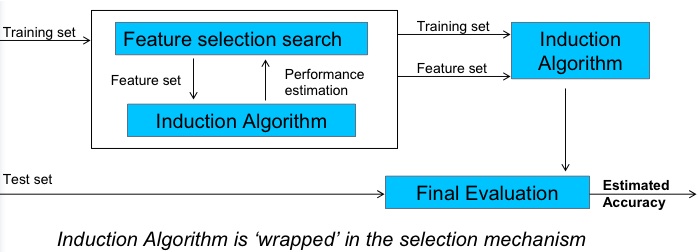
• 10 times, take 90% of the date and run a WRAPPER- a best first search through combinations of attributes. At each step, linear regression was called to asses a particular combination of attributes. In those ten experiments, WRAPPER found that adding feature X to features A,B,C,... improved correlation the following number of times:

  number of folds (%)  attribute
             2( 20 %)     1 S1
             0(  0 %)     2 S2
             2( 20 %)     3 S3
             1( 10 %)     4 S4
             0(  0 %)     5 S5
             1( 10 %)     6 S6
             6( 60 %)     7 S7     <==
             1( 10 %)     8 F1
             1( 10 %)     9 F2
             2( 20 %)    10 F3
             2( 20 %)    11 D1
             0(  0 %)    12 D2
             5( 50 %)    13 D3     <==
             0(  0 %)    14 D4
             0(  0 %)    15 T1
             1( 10 %)    16 T2
             1( 10 %)    17 T3
             1( 10 %)    18 T4
             0(  0 %)    19 P1
             1( 10 %)    20 P2
             0(  0 %)    21 P3
             1( 10 %)    22 P4
             6( 60 %)    23 P5     <==
             1( 10 %)    24 P6
             2( 20 %)    25 P7
             1( 10 %)    26 P8
             0(  0 %)    27 P9
             2( 20 %)    28 Hours
             8( 80 %)    29 KLoC   <==
             4( 40 %)    30 Language
             3( 30 %)    32 log(hours)
  

• Four variables appeared in the majority of folds. A second run did a 10-way using just those variables to yield a smaller model with (much) larger correlation (98\%):

  Defects =
      876.3379 * S7=VL +
     -292.9474 * D3=L,M +
      483.6206 * P5=M +
        5.5113 * KLoC +
       95.4278
  

Excess attributes

• Confuse decision tree learners
  • Too much early splitting of data
  • Less data available for each sub-tree
• Too many things correlated to class?
  • Dump some of them!

Why FSS?

• throw away noisy attributes
• throw away redundant attributes
• smaller model= better accuracies (often)
• smaller model= simpler explanation
• smaller model= less variance
• smaller model= any downstream processing will thank you

Problem

• Exploring all subsets exponential
• Need heuristic methods to cull search;
  • e.g. forward/back select

• Forward select:

  • start with empty set
  • grow via hill climbing:
  • repeat
    • try adding one thing and if that improves things
    • try again using the remaining attributes
  • until no improvement after N additions OR nothing to add

  • Back select

  • as above but start with all attributes and discard, don't add

  • Usually, we throw away most attributes:

  • so forward select often better

  • exception: J48 exploits interactions more than,say, NB.
  • so, possibly, back select is better when wrapping j48
  • so, possibly, forward select is as good as it gets for NB

Supervised vs Unsupervised

• Supervised, use the class variable in column2 to discretize column1.
  • E.g. split column1 such that the etropy of the column2 symbols are minimized.
  • see below
• Unsupervised, just refect on column1.
  • E.g. find splits that minimize the variance afer the spits.

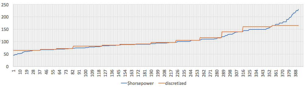
E.g. here unsupervised discretization running on the horsepower column of auto.csv. Note these numbers run 46 to 230 and this code](http://menzies.us/lean/unsuper.html) decides that this should be divided into:

• less that 65
• 66 to 69
• 69 to 72
• 74 to 82
• 83 to 86
• 87 to 89
• 90 to 91
• 92 to 97
• 98 to 105
• 107 to 116
• 120 to 140
• 142 to 160
• over 165

46.. 230
|.. 46.. 116
|.. |.. 46.. 82
|.. |.. |.. 46.. 65 (..65)
|.. |.. |.. 66.. 82
|.. |.. |.. |.. 66.. 72
|.. |.. |.. |.. |.. 66.. 69 (66..69)
|.. |.. |.. |.. |.. 69.. 72 (69..72)
|.. |.. |.. |.. 74.. 82 (74..82)
|.. |.. 83.. 116
|.. |.. |.. 83.. 97
|.. |.. |.. |.. 83.. 91
|.. |.. |.. |.. |.. 83.. 86 (83..86)
|.. |.. |.. |.. |.. 87.. 91
|.. |.. |.. |.. |.. |.. 87.. 89 (87..89)
|.. |.. |.. |.. |.. |.. 90.. 91 (90..91)
|.. |.. |.. |.. 92.. 97 (92..97)
|.. |.. |.. 98.. 116
|.. |.. |.. |.. 98.. 105 (98..105)
|.. |.. |.. |.. 107.. 116 (107..116)
|.. 120.. 230
|.. |.. 120.. 160
|.. |.. |.. 120.. 140 (120..140)
|.. |.. |.. 142.. 160 (142..160)
|.. |.. 165.. 230 (165..)

FSS types:

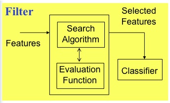
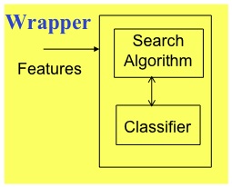
• filters vs wrappers:

  • wrappers: use an actual target learners e.g. WRAPPER
  • filters: study aspects of the data e.g. the rest
  • filters are faster!
  • wrappers exploit bias of target learner so often perform better, when they terminate
    • don't terminate on large data sets

  • solo vs combinations:

  • evaluate solo attributes: e.g. INFO GAIN, RELIEF

  • evaluate combinations: e.g. PCA, SVD, CFS, CBS, WRAPPER
  • solos can be faster than combinations

  • supervised vs unsupervised:

  • use/ignores class values e.g. PCA/SVD is unsupervised, reset supervised

  • numeric vs discrete search methods

  • ranker: for schemes that numerically score attributes e.g. RELIEF, INFO GAIN,

  • best first: for schemes that do heuristic search e.g. CBS, CFS, WRAPPER

Hall and Holmes:

This paper: pre-discretize numerics using entropy.

Hall & Holmes

INFO GAIN

• often useful in high-dimensional problems
  • real simple to calculate
• attributes scored based on info gain: H(C) - H(C|A)
• Sort of like doing decision tree learning, just to one level.

RELIEF

• Kononenko97
• useful attributes differentiate between instances from other class
• randomly pick some instances (here, 250)
• find something similar, in an another class
• compute distance this one to the other one
• Stochastic sampler: scales to large data sets.

• Binary RELIEF (two class system) for "n" instances for weights on features "F"

  set all weights W[f]=0
  for i = 1 to n; do
     randomly select instance R with class C
     find nearest hit H      // closest thing of same class
     find nearest miss M     // closest thing of difference class
     for f = 1 to #features; do
         W[f] = W[f] - diff(f,R,H)/n + diff(f,R,M)/n
     done
  done
  

• diff:

  • discrete differences: 0 if same 1 if not.
  • continuous: differences absolute differences
  • normalized to 0:1
  • When values are missing, see Kononenko97, p4.

• N-class RELIEF: not 1 near hit/miss, but k nearest misses for each class C

  W[f]= W[f] - ∑i=1..k diff(f,R, Hi) / (n*k)
             + ∑C ≠ class(R) ∑i=1..k (
                                  P(C) / ( 1 - P(class(R)))
                                  * diff(f,R, Mi(C)) / (n*k)
                                 )
  

  The P(C) / (1 - P(class(R)) expression is a normalization function that

  • demotes the effect of R from rare classes
  • and rewards the effect of near hits from common classes.

CBS (consistency-based evaluation)

• Seek combinations of attributes that divide data containing a strong single class majority.
  • Kind of like info gain, but emphasis of single winner
• Discrete attributes
• Forward select to find subsets of attributes

WRAPPER

• Forward select attributes
  • score each combination using a 5-way cross val
• When wrapping, best to try different target learners
  • Check that we aren't over exploiting the learner's bias
  • e.g. J48 and NB

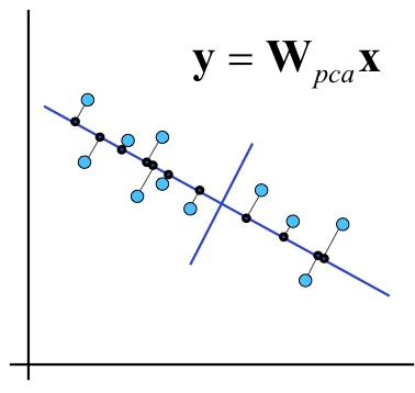
PRINCIPAL COMPONENTS ANALYSIS (PCA)

(The traditional way to do FSS.)

• Only unsupervised method studied here
• Transform dimensions
• Find covariance matrix C[i,j] is the correlation i to j;
  • C[i,i]=1;
  • C[i,j]=C[j,i]
• Find eigenvectors
• Transform the original space to the eigenvectors
• Rank them by the variance in their predictions
• Report the top ranked vectors

• Makes things easier, right? Well...

  if   domain1  <= 0.180
  then NoDefects
  else if domain1 > 0.180
       then if domain1 <= 0.371 then NoDefects
       else if domain1 > 0.371 then Defects
  
  domain1 = 0.241 * loc     + 0.236 * v(g)
          + 0.222 * ev(g)   + 0.236 * iv(g)     + 0.241 *  n
          + 0.238 * v       - 0.086 * l         + 0.199  * d
          + 0.216 * i       + 0.225 * e + 0.236 * b + 0.221  * t
          + 0.241 * lOCode  + 0.179 * lOComment
          + 0.221 * lOBlank + 0.158 * lOCodeAndComment
          + 0.163 * uniqO p + 0.234 * uniqOpnd
          + 0.241 * totalOp + 0.241 * totalOpnd
          + 0.236 * branchCount
  

CFS (correlation-based feature selection)

• Scores high subsets with strong correlation to class and weak correlation to each other.
• Numerator: how predictive
• Denominator: how redundant
• FIRST ranks correlation of solo attributes
• THEN heuristic search to explore subsets

And the winner is:

• Wrapper! and it that is too slow...
• CFS, Relief are best all round performers
  • CFS selects fewer features
• Phew. Hall invented CFS

Instance Selection

Prototype Selection with Clusters

• Step1: Feature selection: sort columns by their Infogain score. Delete bottom half.
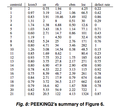
• Step2: Cluster: return one example pre centroid.

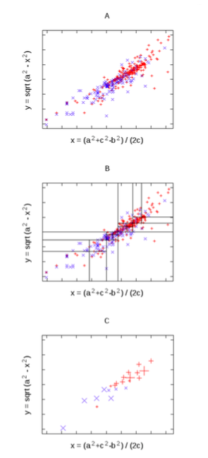
Reduction of 800 rows by 24 attributes to 5 attributes by 22 rows

For many data sets:

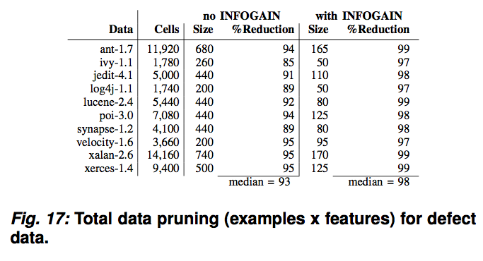
Note that for classification by weighted scores from 2 nearest neighbors, the reduced data as accurate as the full data.